In this post I rewrite some notes from my game theory course to solve the “how much should you bid” Riddler.
Problem set-up: Going once, going twice (you’re still on this page??? well then buckle up, it’s time for some game theory)
The premise for the problem is you are bidding against your arch-rival for a painting. You each have a valuation for the painting drawn from a uniform distribution between 0 and 100,000,000. You each submit a sealed bid (private valuation), with a winner pay format, first price format.
Formal like a tuxedo t-shirt
What is the object we are looking for? Well, for this sort of game we want a Bayesian Nash Equilibrium. For completeness, I’ll briefly mention what a Nash EQ is before defining a BNE. The core principle behind a NE (despite what a certain movie might have you believe…) is that all players are playing strategies that are best responses to the strategies played by all of the other players. That is there is no profitable unilateral deviation (i.e. no one player can do better by playing a different strategy unless the other players were to also change their strategies).
The Bayesian version of this concept isn’t so different, but since we’re being all Bayesian about things know we’ve got beliefs floating around. These beliefs will be driven by Nature (Harsanyi 1967), which is basically a short-hand way of modeling randomness in the game. The important thing for these Bayesian games is that there is some sort of incomplete information. Being lazy and taking the definition from wikipdia… “A Bayesian Nash equilibrium is defined as a strategy profile and beliefs specified for each player about the types of the other players that maximizes the expected payoff for each player given their beliefs about the other players’ types and given the strategies played by the other players.”
But since I’m studying for prelims… let’s practice making this a bit more formal. I’m going to follow Mas Collel, Whinston, & Green for this, but there are plenty of similar notes online. A Bayesian game has the following elements:
- players { 1, … , i , … , N }
- payoff function: \(u_i(s_i, s_{-i}, \theta_i)\)
- player type: \(\theta_i \in \Theta_i\) player type for player i chosen by nature (private information to i)
- Joint pdf of \(\theta_i\)’s governed by a (commonly) known \(F(\theta_i,...,\theta_N)\)
- strategies (read: decision rule), \(s_i(\theta_i)\in S_i\), importantly a function of player type.
We can thus summarize the game as \([N, \{S_i\}, \{ u_i(\cdot) \}, \Theta, F(\cdot)]\). With this in mind, it is easy to formulate the definition of an equilibrium as: the set of decision rules \((s_1(\cdot),...,s_N(\cdot))\) s.t. \(\mathbb{E}[u_i(s(\theta),\theta)]\geq \mathbb{E}[u_i(s'_i(\theta_i),s_{-i}(\theta_{-i}),\theta)\). Another way of framing this is to say a profile of decision rules is a BNE iff \(\mathbb{E}_{\theta-1}[u_i(s_i(\tilde{\theta}_i),s_{-i}(\theta_{-i},\tilde{\theta}_i)|\tilde{\theta_i}]\geq \mathbb{E}_{\theta-1}[u_i(s'_i,s_{-i}(\theta_{-i},\tilde{\theta}_i)|\tilde{\theta_i}] \forall s'_i \in S_i.\) This definition tells us that we can basically treat each type of player seperately, with each rying to max her payoff given the conditional pd over her rivals choices.
No go or Van Gogh
Let’s map the riddle into our framerwork. For the basic level of the riddle we have N=2, two players– but since I’m assuming some of have more than one arch-nemesis at a time, I’m actually going to solve the expanded case simultaneously so let’s not focus to much on this, so no worries if you like to maintain a group of nemeses (I’m gonna go ahead and label a group of nemeses a murder ‘cause that seems about right). We have a value function \(u(\theta_i)=\theta_i\) and \(\theta_i\) is drawn from our uniform PDF (CDF) f (F) from 0 to 100,000,000. Let’s just guess a random strategy to get a sense for how things might play out. A natural one is to bid your type. This yields a value of 0 no matter what happens, since if you lose you pay nothing but get nothing and if you win you pay all the value you just won! I bet we can do better…
For instance, here is a dumb proof the above strategy is dominated. Let’s say I bid my value minus epsilon. Then my expected value is the probability that I win times the value I get from winning, or \(P(\theta_i-\epsilon>\theta_{-i})*(\theta-(\theta_i-\epsilon)).\) This is clearly a positive value, so we have a profitable one shot deviation.
All right, so our first guess didn’t work out, let’s think a bit harder about what we should do with this epsilon type argument. Sure it seems to work for a tiny number, but if let epsilon go to theta thats not going to do us much good either, since we’ll never win \(P(\theta_i-\epsilon>\theta_{-i})\rightarrow 0.\) Hmmm….
Outsmart your rival (or I guess equally smart your rival?)
No matter how much it annoys us to a admit it, maybe you are and your rival aren’t so different. In fact, you both have the same value function, and are drawing you types from the same underlying distribution. This seems to hint that the two of you will play the same the strategy. So let’s guess that will be the case and then verify.
Our strategy will be as follows. Let all players except the first play strategy B where \(B_i:[0 \quad 100,000,000] \rightarrow \mathbb{R}_+\) Without loss of generality let’s assume B is increasing and differentiable. Basically, this just means that our bidders are bidding more when they value the art more, and they aren’t jumping around too much when they are doing so. Not so crazy…
The goal will be to show that player 1 (an arbitrary player) best response includes B. This will then confirm that B is our BNE strategy. Lets get some notation and facts out of the way. When player 1 is of type \(\theta\) then \(B(\theta_1)=b\) just means that player 1 bids b when he values the art at \(\theta\). Not so bad! What else do we know about B? Well, if I don’t value the art at all (and let’s be honest, I have bad taste in art so that probably happens far more often than I care to admit…) then I probaly don’t want to bid anything, since I’d prefer to keep my cash and forgo the Van Gogh, so \(B(0)=0\). Bidder 1 wins when her bid is higher than everyone elses, ie. \(max_{i\neq 1} B(\theta_i)\leq b\) Since B is increasing we can go ahead and move our max operator into the function (this should seem natural to you hopefully, everyone is bidding more when they value more so the maximum bid placed by your opponents is just the bid placed by your opponent with the highest valuation. That means \(max_{i\neq 1}=B(max_{i\neq 1}\theta_i)=B(y_1)\) Where the last equality is just how I’m going to define y for notational simplicity \((y_1=max{v_2,...,v_N}\). So bidder 1 wins when \(y_1 \leq B^{-1}(b).\) I’m not saying anything suprising with this line, it’s basically just saying when player 1 bids the most she wins, but it ties this concept explicitly to her opponent with the highest valuation.
So let’s write this down as a generic maximazation problem for player 1 with type \(\theta\). What are we maximizing? Well hopefully our previous work makes this clear, our chance of being the highest bidder (which clearly depends on our bid), and the amount we get from winning (also depends on our bid), and the only thing we are choosing is what we bid: \(max_{b\geq 0} G(B^{-1}(b))(\theta-b)\). Where G is the CDF of \(y_1\), g will be the pdf.
Let’s see how well we remember our calc 1 and take the first order condition and set it equal to 0: \(\frac{g(B^{-1}(b))}{B'(B^{-1}(b))}(\theta-b)-G(B^{-1}(b))=0\) Basically just remember your chain rule and that \(\frac{d}{db} B^{-1}(b)=\frac{1}{B'(B^{-1}(b))}\).
This is a bit ugly, let’s see if we can exploit our symmetry a bit more. Remember that \(B(\theta)=b\) so \(B^{-1}(b)=\theta\). So the foc is actually \(G(\theta)B'(\theta)+g(\theta)B(\theta)=\theta g(\theta)\). But this should look pretty familiar, its just \(\frac{d}{d\theta}(G(\theta)B(\theta))=\theta g(\theta)\) Let’s remember we just want to solve for \(B(\theta)\) but that’s no problem now. So algebra yada-yada and we get the symmetric BNE \(B(\theta)=\frac{1}{G(\theta)}\int_0^\theta y g(y) dy\). This satisfies all our initial assumations and turns out to be just the exepectation of \(y_1\) conditional of it being less than \(\theta\) (or in words, the expected value of second highest type conditional on player 1’s type being the highest).
I guess we should actually write down a solution now
So, fun fact, I made this way harder than what we needed for this problem. We’ve actually solved this problem for a whole bunch of possible distribution functions (cool right?). But now we can just plug and chug for our problem, which uses a uniform distribution. It turns out that \(G(\theta_1)=(\frac{\theta_1}{100,000,000})^{N-1}.\) Let’s take a second to interpret this: since we have i.i.d draws from the distribution, the probability that player 1’s value is the highest is just the probability that her value is higher than player 2, times the probability that her value is higher than player 3, times… well you get it, which means the pdf, g is \(\frac{(N-1)}{100,000,000}(\frac{\theta_1}{100,000,000})^{N-2}\). So putting that all together, our answer is:
\(B(\theta)=(\frac{\theta_1}{100,000,000})^{N-1}\int_0^\theta y \frac{(N-1)}{100,000,000}(\frac{y}{100,000,000})^{N-2} dy\)
\(B(\theta)=(\frac{\theta_1}{100,000,000})^{N-1} * \frac{100,000,000(N-1)}{N}[(\frac{y}{100,000,000})^{N}]^\theta_0\)
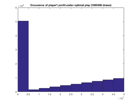
Which gives us our final answer: \(B(\theta)=\frac{(N-1)}{N}\theta\)
So when you’re bidding against just your rival you want to bid one-half of how much you value the painting. Here’s what your profits look like playing this strategy over a large number of draws.
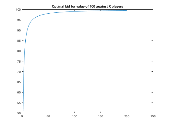
As N get larger you bid closer and closer to your value. Here’s what optimal play looks like as you increase your number of opponents holding your value constant.
FYI: these slides are very good on this subject.
You scream, I scream, we all scream for all-pay
Sure we’ve had analysis under one auction rule, but what about a second auction rule? Let’s just go ahead and make everyone pay, regardless of whether they win. Let’s take a look at the all pay auction. Since we’ve already done most of the work here I’m going to be a little bit less wordy for this part.
The all pay setting doesn’t actually change things all too much. Again we’re going to look for identical, increasing functions. The payoff for player i is now \(\theta_iF^{N-1}(B_j^{-1}(b_i))-b_i\). This is almost the same as before, except the probability distribution no longer is hitting the bid, since the player has to pay it regardless. Lets take a first order condition with respect to b:
\[\theta_i(N-1)[F(B_j^{-1}(b_i))]^{N-2}\frac{f(B_j^{-1}(b_i))}{B'_j(B_j^{-1}(b_i))}-1=0\]Let’s use the same trick with \(B(\theta)=b\) so \(B^{-1}(b)=\theta\)
So we can write: \(\theta (N-1) F(\theta)^{N-2} \frac{f(\theta)}{b'(\theta)}-1=0\)
\[b'(\theta) = \theta (N-1) F(\theta)^{N-2}f(\theta)\] \[b(\theta) = (N-1) \int_0^\theta yF(y)^{N-2}f(y) dy\]But we know, \(F(y)=\frac{x}{100,000,000}, f(y)=\frac{1}{100,000,000}\) so
\[(N-1)\int_0^\theta y*(\frac{y}{100,000,000})^{N-2}*\frac{1}{100,000,000}\] \[b(\theta) = \frac{(N-1)\theta^N}{N*100,000,000^{N-1}}\]